Semantic Image Clustering with CLIP

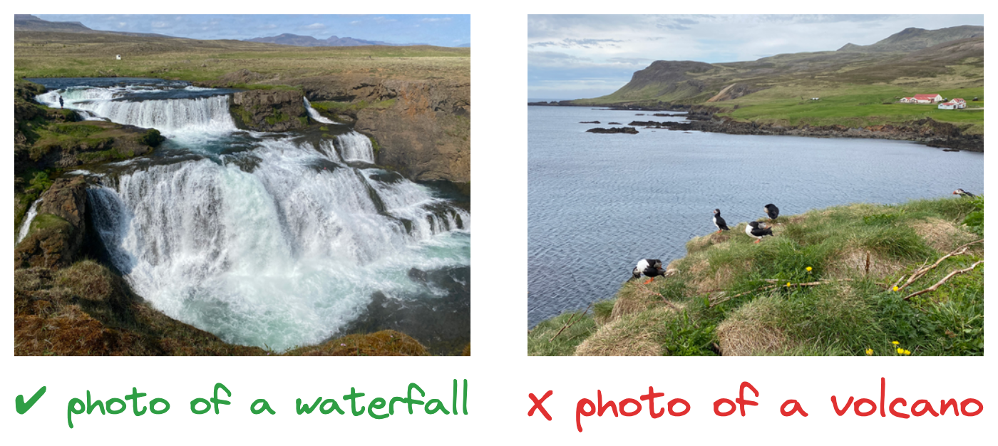
When DALL-E 2 was released to the public last year, it instantly became a hit. Its ability to generate imaginative and unique images from text prompts captured not only AI enthusiasts, but arguably also catalysed the formation of a community centred around generative AI. Beyond its image generation prowess, DALL-E's image understanding capabilities were driven by CLIP, a powerful cross-modal model. In this post, we will explore the lesser-known but equally impressive non-generative aspects of CLIP, focusing on its applications in semantic image clustering.
To begin, we will have a look at the model architecture of CLIP and how it is trained. Then, we will see how a trained CLIP model can be used for image clustering. We will also discuss the additional algorithms needed for this approach. Lastly, we will go through the code to see how well this clustering method works on a real dataset, determining how accurately it groups images based on their similarity.
Introduction to CLIP
To understand the need for CLIP (Contrastive Language–Image Pre-training), we first need to consider how image classifier models – i.e., conventional image understanding models are trained. These models are typically trained in a supervised fashion on large, human-annotated datasets with a finite number of labels. Since the datasets are human-annotated, it is quite expensive to annotate a dataset large enough to be useful for training. Furthermore, the models cannot predict beyond the finite number of labels seen during training, and fine-tuning is required for adding any additional capabilities.
While CLIP is a cross-modal model, and not merely a classifier, it addresses both of the aforementioned issues with image classifier training. Instead of depending on human-annotated datasets, CLIP is trained on pairs of images and text collected from open internet sources. During its training, CLIP aims to maximize a similarity score for correct pairs (i.e., matching images and text) and minimize it for incorrect pairs (i.e., mismatching images and text).
The result is a versatile model that can relate text to images and vice versa. For example, CLIP can be used as an image classifier by ranking a number of labels against an image, even if it has not seen the specific label during training (i.e., zero-shot learning).
Architecture
Under the hood, CLIP employs a text encoder and an image encoder. These encoders, given either text or an image, output a fixed-size numerical vector representation. During training, the encoders are jointly optimized as they learn to associate similar text and image pairs. This process enables CLIP to understand the relationships between text phrases and visual content, bridging the gap between language and vision. This concept is visually depicted in the diagram below.
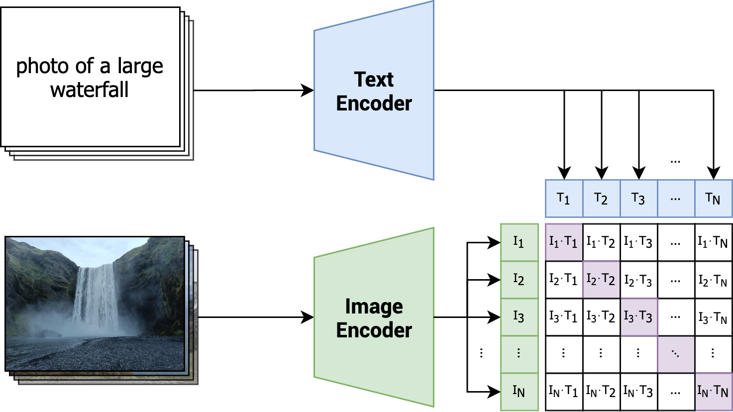
With each iteration of training, the CLIP model is presented with a batch comprising N pairs. Each pair is composed of an image and its corresponding text. The model's learning objective revolves around enhancing the similarity among related pairs (indicated by diagonal, purple cells), while concurrently diminishing the similarity between unrelated pairs (indicated by remaining white cells). This contrasting mechanism characterizes CLIP as contrastive: it acquires meaningful representations by discerning positive (similar) pairs from negative (dissimilar) pairs.
Utility of Embeddings
As previously discussed, the output of the text and image encoders consists of fixed-size numerical vector representations. These vectors are typically referred to as embeddings, and we will refer to them as such in the remainder of this post. These embeddings find application in various downstream tasks, including image classification and clustering. Given CLIP's inherent capacity to discern semantic likeness between images and texts, it is reasonable to expect that the embeddings for an image and its corresponding textual description would display closeness within the embedding space. The same applies to similar image pairs.
In practice, CLIP-generated embeddings are of high dimensionality, usually comprising hundreds or even thousands of dimensions. For the sake of illustration, let us consider two-dimensional representations for a set of images – these embeddings can be visualized as shown below.
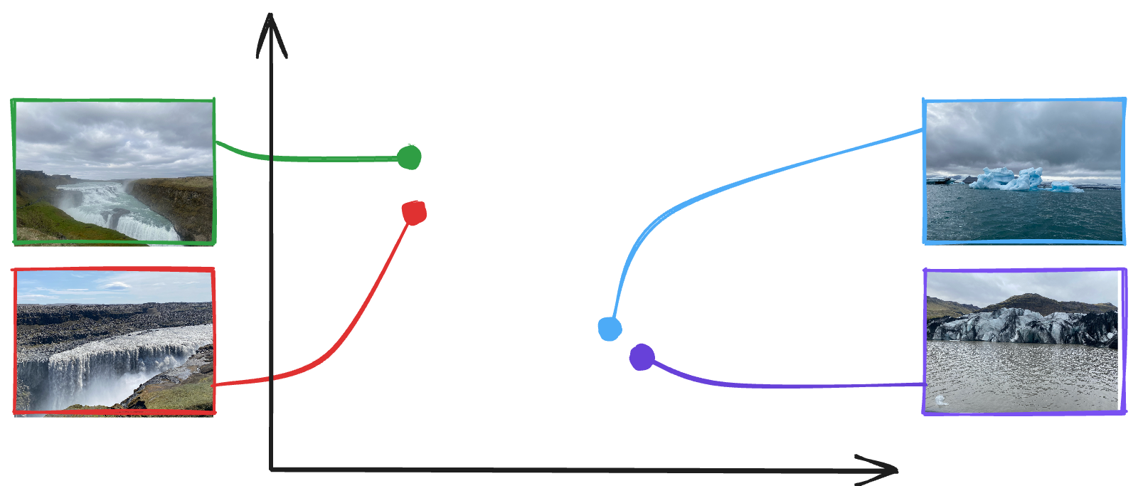
As seen in the visualization, the two waterfall images on the left are proximate to one another in the embedding space, just as the iceberg and glacier images on the right. In a more general sense, any pair of images from a collection can be taken, and their similarity can be quantified. This ability is what enables us to cluster images.
A Clustering Architecture
While we have a similarity measurement for images, we are still missing a component to do the actual clustering. This is not much different from clustering any other vectorized data, such as customer profiles or real estate. The underlying principle involves grouping together similar data points based on their embeddings in a way that minimizes the intra-cluster distance while maximizing the inter-cluster distance.
In theory, we could input the generated CLIP embeddings directly into an off-the-shelf clustering implementation, such as k-means or hierarchical clustering. Unfortunately, this would not provide very useful results. The high dimensionality of the CLIP-generated embeddings makes for less meaningful distance metrics between images, a phenomenon commonly known as the curse of dimensionality.
To understand this phenomenon, imagine you are tasked with clustering houses based on two variables, e.g., square footage and distance from a nearby city. You could easily draw this two-dimensional representation, and use the line distance between points as a similarity measure, as illustrated below.
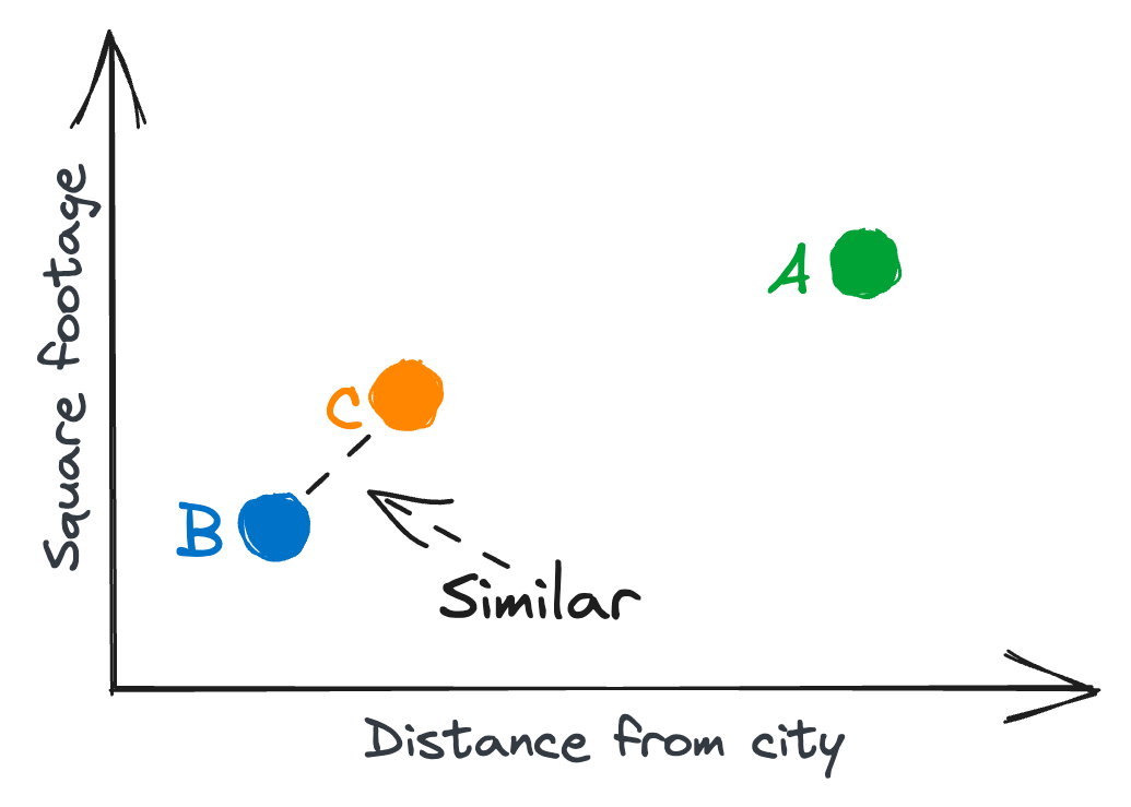
Now, as more features are added to the house representation, the dimensionality increases. For example, you could additionally consider the age of the house, number of bedrooms, and number of bathrooms, bringing the representation to a five-dimensional space. Generally, as the dimensionality grows, the houses (data points) start to spread out across this higher-dimensional space. This can make it difficult to find meaningful patterns or similarities between houses, as the distance between data points tends to converge.
In the case of CLIP, the high dimensionality is the very thing that allows it to capture intricate relationships and nuances within images and their corresponding text descriptions. How can we then retain these nuances while facilitating a meaningful clustering of the data?
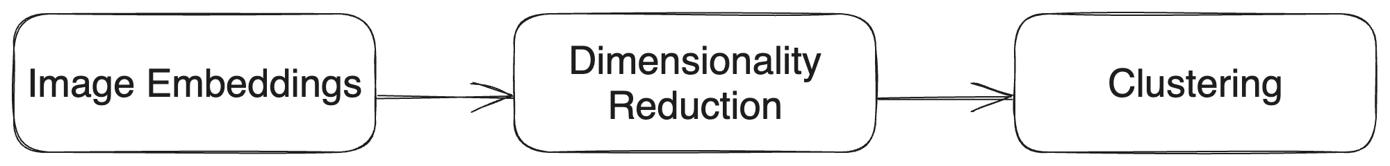
To keep the intricate details of the high-dimensional CLIP embeddings while making clustering meaningful, we can use dimensionality reduction techniques such as PCA or UMAP. These methods shrink the embeddings into a simpler (i.e., lower dimensionality) form that traditional clustering methods can handle better. This way, we balance between capturing the data's complexity and making clustering work effectively in a more manageable space. A high level architecture of the clustering approach, including dimensionality reduction, is depicted below.
Choice of Clustering Algorithm
We previously discussed k-means and other clustering methods, but selecting the appropriate algorithm for implementation raises the question of the optimal choice. While there is no universal solution for clustering, we can establish criteria for selecting a suitable algorithm.
The algorithm should not necessitate the upfront definition of the number of clusters: In many real-world scenarios, identifying the ideal cluster count proves challenging due to diverse data characteristics. Despite k-means being a popular choice, it is not suitable for this context. K-means requires specifying the number of clusters beforehand, which is a limitation given the challenges in determining the optimal cluster count in our scenario.
One promising alternative we explore is HDBSCAN (Hierarchical Density-Based Spatial Clustering of Applications with Noise). It is a density-based clustering algorithm that automatically determines the number of clusters in data without requiring a predefined cluster count. HDBSCAN connects data points based on local density, forming a hierarchy referred to as a "condensed tree," revealing clusters at different levels of detail. HDBSCAN proves robust to noise and outliers, accommodates varying cluster shapes and sizes, and automates the selection of meaningful clusters.
Image Clustering of Iceland
This post would be incomplete without an example of clustering, and a more specific use case of the semantic image clustering. Specifically, we will see how the approach performs on 2,100 pictures taken on a trip to Iceland. Our approach to clustering the images will meticulously follow the same procedure outlined in the earlier section on clustering architecture. Without further ado, let us delve into some code.
Generating Embeddings
While OpenAI has openly provided us with a model architecture, they do not supply any models or code we can use to run the model. Thankfully, we can use OpenCLIP, which provides an open source implementation of CLIP with several models available. Specifically, we will use a model trained by LAION which, at the time of writing, achieves the highest top-1 zero-shot accuracy on ImageNet. Let us first import this model accordingly.
Following the import, we can directly provide images loaded through PIL to CLIP's processor, providing us with embeddings of all images.
In the code above, all files in the ./images path are loaded with PIL and assumed to be images. Generating embeddings for all images can take a while, and you could wrap the image paths with tqdm to monitor progress of the embedding generation. Nevertheless, the snippets above all we need to generate the embeddings, allowing us to move onto dimensionality reduction.
Dimensionality Reduction
As previously mentioned, you could plug in any dimensionality reducing model such as PCA or UMAP at this point. You could try both, or even others, to see how well they fare against each other; in this particular post, we will be using UMAP. Shown below, we specify UMAP to use five components (n_components), which brings our embeddings down to a five-dimensional space.
If you decide to do a clustering only your own, do try different dimensionalities. You could also remove the dimensionality reduction step altogether to recognise the importance of it – in my case, this created a cluster of all images, which fits the theory on the curse of dimensionality.
Clustering
Moving on from dimensionality reduction, the last step before we can begin to analyse our clusters is the actual detection of them. As previously mentioned, we will be using HDBSCAN for this task. As per the implementation's advice, we should be able to detect a good clustering by adjusting only the minimum cluster size. We will set it to 20, corresponding to around 1% of the total dataset.
Simple as that, we now have everything needed to analyse the clusters.
Analysis
From the 2,100 images, 25 unique clusters were identified, and a cluster was found for 92% of images. This percentage depends on the minimum cluster size set previously, and whether the embeddings are cohesive in general. The remaining 8% can be interpreted as more unique images that did not belong in a group with 19 similar images. While we will not go over all 25 clusters, below we shall take a look at a selection of clusters.
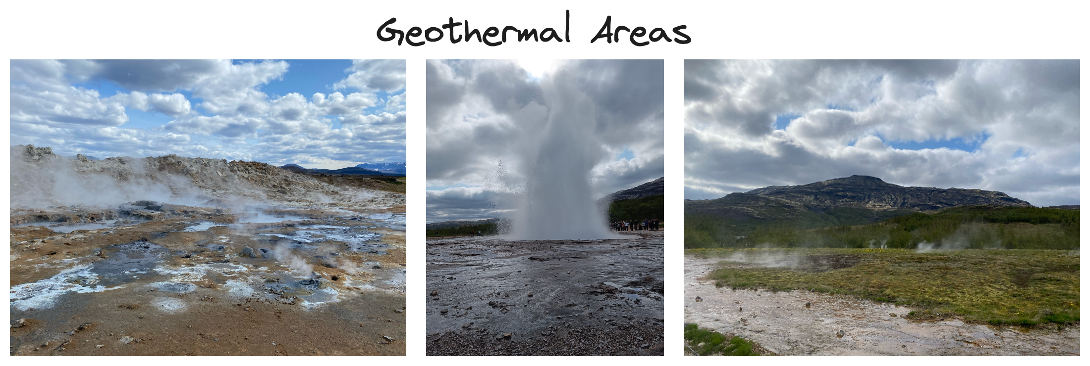
The album contains several images taken in the geothermal areas in southern Iceland (i.e., where Geysir is located), as well as the northern geothermal areas. While these areas are geologically similar, they are visually dissimilar. Impressively, the model managed to pick up on the relation between the areas.
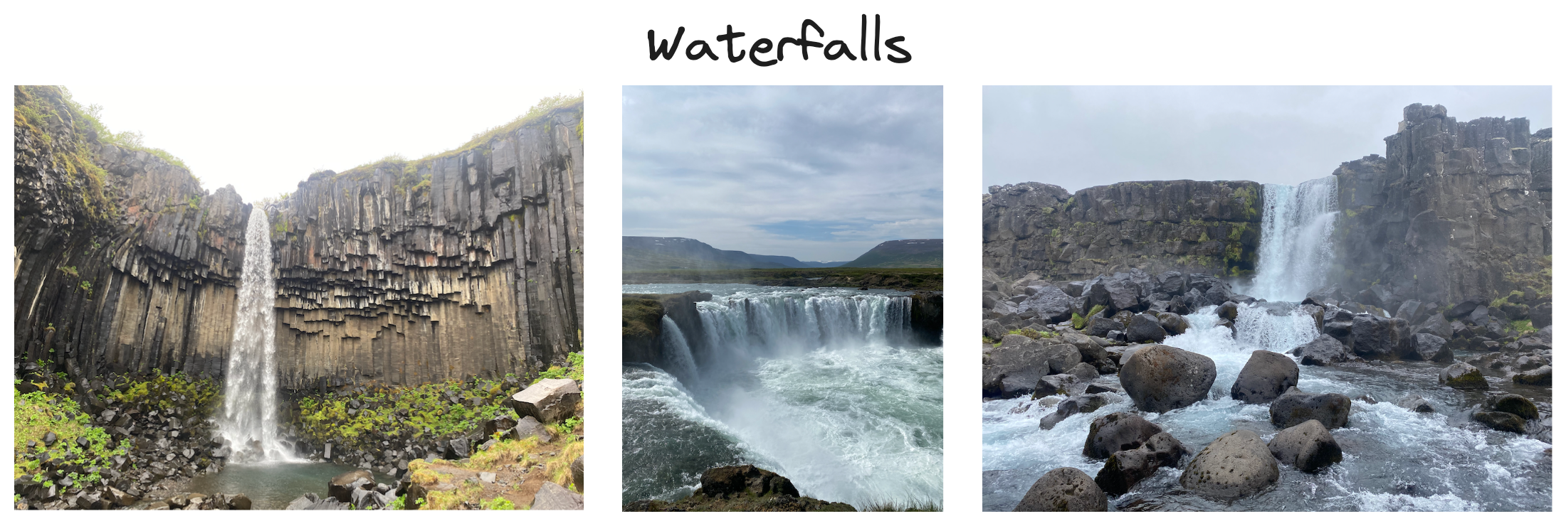
Waterfalls undoubtedly make up the majority of images in the album, so it would be a surprise if they did not form a cluster. Interestingly, the waterfalls in this dataset are split in several clusters: pictured above is the biggest cluster, containing a variety of waterfalls with few individual images. For individual waterfalls with more images than the threshold, the model has generated individual clusters. We will return to the relation between these clusters later.
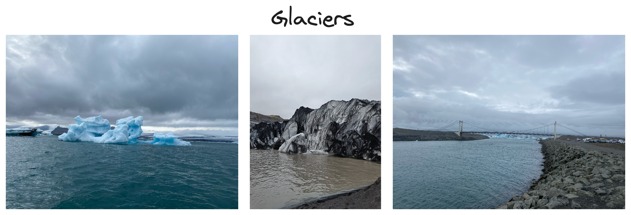
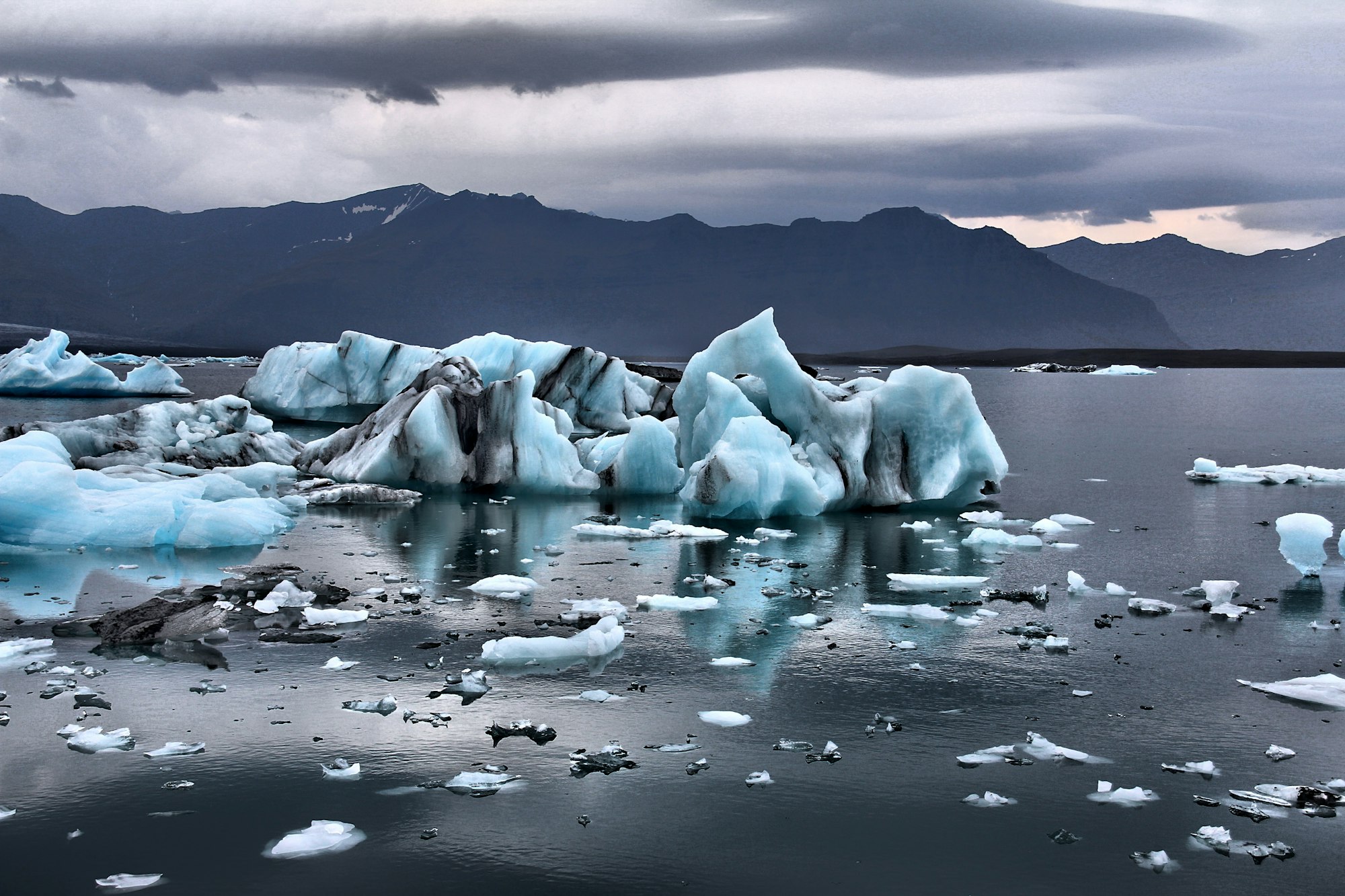
Glaciers are visually distinctive from the other images in the album, so it is not surprising that the few pictures in the album were enough to cluster. Interestingly, the glacier lagoon on the right of the excerpt above is barely visible, yet the model still identified that it is related to glaciers.
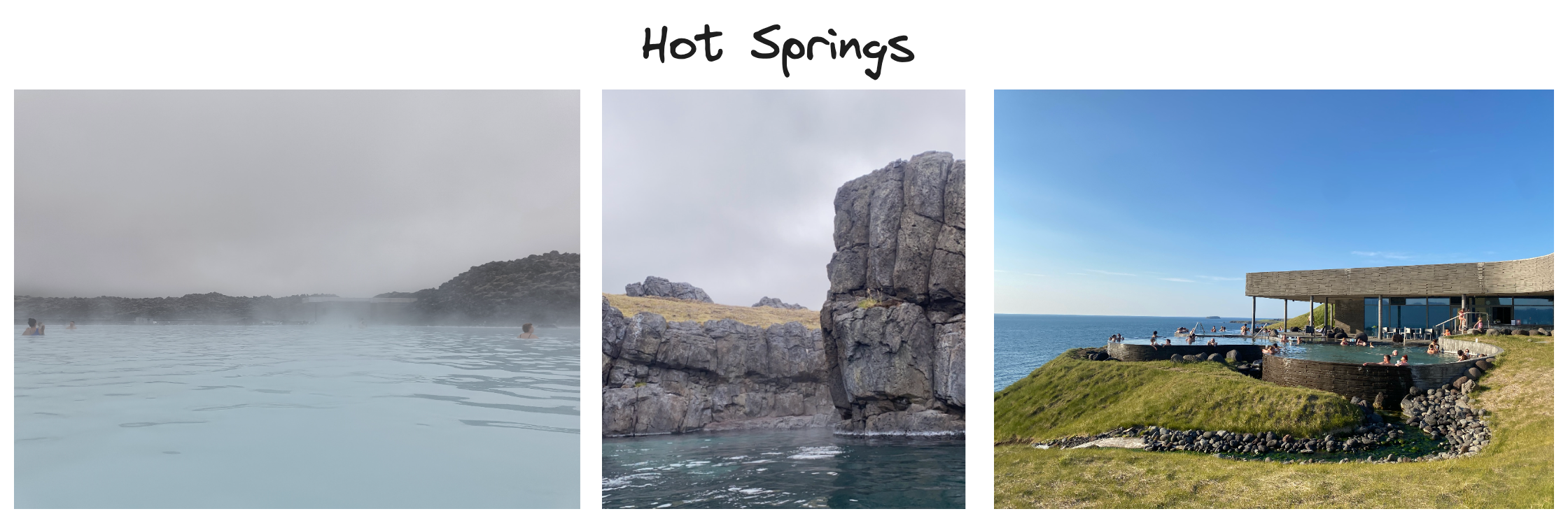
The model managed to identify a cluster of all images taken at various hot springs in Iceland. Visually, these images are similar to other images in the album taken in open waters and at coasts, so the model's distinction between the groups is quite impressive. As seen above, the model also managed to group images taken inside and outside the hot springs.
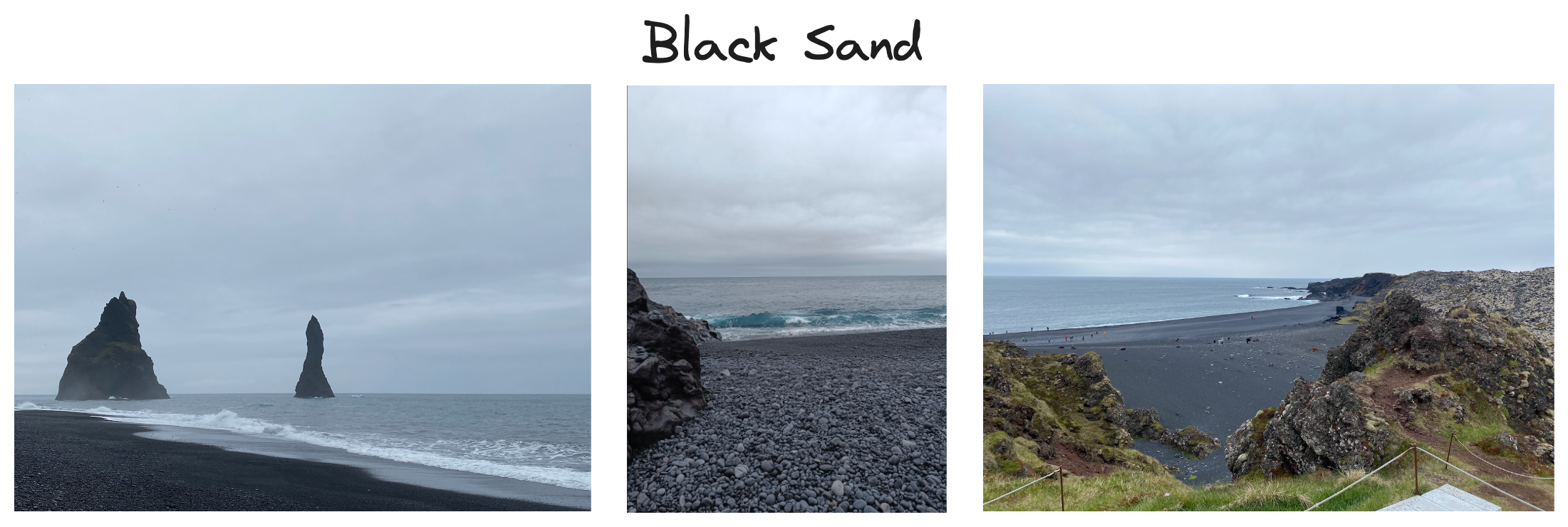
Iceland is well known for its black sand beaches, caused by the volcanic activity on the island. In this case, the model detected a group of images with the common feature being black sand. Arguably, the pictures above could be labelled as coast, but the model made a separate cluster where only coastline is present without black sand. As we shall see soon, these two clusters are somewhat related.
Plotting the Clusters
Clearly, the model is able to identify some meaningful clusters across all the input images. However, the clusters alone provide little insight into the rationale behind the clusters, and how they are related to each other. For instance, one could imagine that scorching geothermal areas and icy glaciers represent semantic opposites, whereas hot springs are intuitively more closely associated with phenomena like geothermal areas.
Our five-dimensional data does not lend itself to any meaningful visualizations. To visualize the data meaningfully, we can reduce the embeddings further down to a two-dimensional space. Then, we can plot the data in a scatter plot, each dot representing an image. For simplicity, an excerpt of clusters is shown below. You can hover on an individual point to see which cluster it belongs to.
Interpreting the results, most of the waterfall clusters seem to fall in the lower region of the plot, indicated by the dashed blue line. The exception to this is the Stuðlagil Canyon cluster, whose images carry visual resemblances to the waterfall clusters. Another similar pair is the Coast and Black Sand clusters, encapsulated in the dashed rectangle. Given that black sand images are typically taken at coasts, the short distance between these clusters is reasonable. Regarding the hypothesized example of Geothermal Areas and Glaciers being far apart, there is some merit to it. However, the Geothermal Areas cluster does seem to be an outlier in general, being distant from the majority of clusters.
What's next?
If you decide to experiment with this model or clustering architecture on your own, a logical extension is to include image captioning on the derived clusters. For this purpose, you could employ a model such as BLIP. The captions could be based on the average embedding of the images in the cluster. Alternatively, you could base it on the embeddings of the most central image (i.e., the one that is most similar to the other images in the cluster).
Another direction is to see if you can improve the quality of the clustering by use of different dimensionality reduction techniques, or different clustering algorithms. In this post, we combined UMAP and HDBSCAN, but there is no evidence to support that this combination is superior to any other. You can mix and match these algorithms as you please, or play around with their parameters.
You could also augment the embeddings with auxiliary data, or perform secondary clusterings using such data. For example, pictures taken with smartphones may contain latitude and longitude as part of their metadata. Extracting these locations, you could cluster the images based on their location using an appropriate metric (e.g., Haversine distance).
Finally, if you are wondering if text can be clustered semantically in a similar way, you are in luck. The main source of inspiration for this post is BERTopic, a topic modeling technique based on the same principles of clustering embeddings. Recently, support for multi-modal clustering has been added to the repository, so you can even use BERTopic as a basis for image clustering.